This article is meant to be the last one on this blog, and aims at summing up the ideas developped in the previous articles to give a rather accurate sketch of proof of the asymptotic Goldbach conjecture.
First, let’s give all the relevant notations:
 : a positive integer strictly greater than
  .
.
 : a primality radius of , namely a non-negative integer less than
  such that both
  and
and  are primes.
 : the
: the  -tuple
  , where
  denotes the
  -th prime.
 :
:  where
where  is the number of primes below
  .
.
 : the product of the first primes.
 : the -th potential typical primality radius of , i.e the
  -th non-negative integer less than
  such that both
  and
and  contain no
  :
:
for all prime  less than
  , one has simultaneously:

and

The adjective « typical » means that:

and the adjective « potential » is used because of the upper limit

A potential typical primality radius of less than will be simply called a typical primality radius of .
 : the total number of potential typical primality radii of , an expression of which is:
 .
.
 : the total number of typical primality radii of .
 : the quantity
  .
.
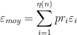
 : the quantity
 if
if 
The quantities  for ranging from
  to will be called « Goldbach gaps of the first kind ».
 : a quantity such that:
if <  then <
and such that there exists such that 
The quantities will be called « Goldbach gaps of the second kind » and the number of such that:
that is, the multiplicity of , will be denoted by  .
.
 : the number of Goldbach gaps of the second kind.
 : the ratio
  .
.
 : the quantity equal to:
 if
if  and equal to otherwise.
 : the quantity
  .
.
 : the ratio
  .
.
The famous Goldbach conjecture asserts that every even integer greater than  is the sum of two primes. We define the number , which depends on , in the following way:
where is the number of primes less or equal to .
 is a prime only if for all prime less or equal to , doesn’t divide .
There are exactly such primes. The number will be called the « natural configuration order » of .
Then we define the « -order configuration » of an integer  , denoted by
  , as the following sequence:
 .
.
For example  .
.
We call  the « natural configuration » of .
An almost sufficient condition to make  be a primality radius of is:
For all integer such that  :
:
 differs from
and
 differs from
If this double statement is true, will be called a « potential typical primality radius » of .
Moreover, if  , then will be called a « typical primality radius » of and denoted simply by .
In what follows we show that every large enough positive integer admits a typical primality radius, from which it follows that every large enough even integer is the sum of two primes.
The proof is based on two lemmas:
Lemma 1: 
Proof:
One has:

But:

 .
.
Using Mertens’ formula, namely:
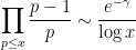
one gets:

and thus:

where

is the so called twin prime constant.
Finally:

hence:
.
Lemma 2: Assume that  .
.
Then  .
.
Proof:
One has:

and:
thus:
Moreover, one has:
so that:

hence:

Hence:

and:

Therefore
Theorem: 
Proof:
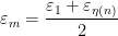
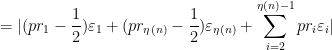
One can use the inequality of the arithmetic and geometric mean to write:

As , one gets:

As obviously  and
and  , one finally gets:

Hence  .
.
All that remains to be done is to prove the inequality , which should be true whenever  . This will be the subject of a future article.

